Training very deep neural networks is hard. It turns out one significant issue with deep neural networks is that the activations of each layer tend to converge to 0 in the later layers, and therefore the gradients vanish as they backpropagate throughout the network.

A lot of this has to do with the sheer size of the network - obviously as you multiply numbers less than zero together over and over, they’ll converge to zero, and that’s partially why network architectures such as InceptionV3 insert auxiliary classifiers after layers earlier on in their network, so there’s a stronger gradient signal back propagated during the first few epochs of training.

However, there’s also a more subtle issue that leads to this problem of vanishing activations and gradients. It has to do with the initialization of the weights in each layer of our network, and the subsequent distributions of the activations in our network. Understanding this issue is key to understanding why batch normalization is now a staple in training deep networks.

First, we can write some code to generate some random data, and forward it through a dummy deep neural network:

n_examples, hidden_layer_dim = 100, 100
input_dim = 1000
X = np.random.randn(n_examples, input_dim) # 100 examples of 1000 points
n_layers = 20
layer_dim = [hidden_layer_dim] * n_layers # each one has 100 neurons

hs = [X] # stores the hidden layer activations 
zs = [X] # stores the affine transforms in each layer, used for backprop
ws = [] # stores the weights

# the forward pass
for i in np.arange(n_layers):
	h = hs[-1] # get the input into this hidden layer
	#W = np.random.randn(h.shape[0], layer_dim[i]) * np.sqrt(2)/(np.sqrt(200) * np.sqrt(3))
	#W = np.random.uniform(-np.sqrt(6)/(200), np.sqrt(6)/200, size = (h.shape[0], layer_dim[i]))
	W = np.random.normal(0, np.sqrt(2/(h.shape[0] + layer_dim[i])), size = (layer_dim[i], h.shape[0]))
	#W = np.random.normal(0, np.sqrt(2/(h.shape[0] + layer_dim[i])), size = (layer_dim[i], h.shape[0])) * 0.01
	z = np.dot(W, h)
	h_out = z * (z > 0)
	ws.append(W)
	zs.append(z)
	hs.append(h_out)

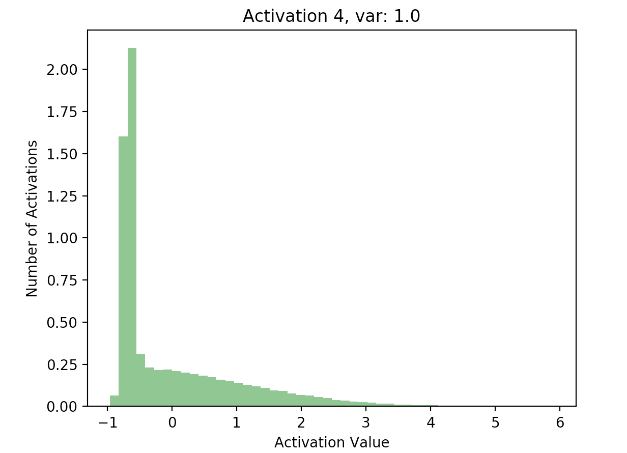
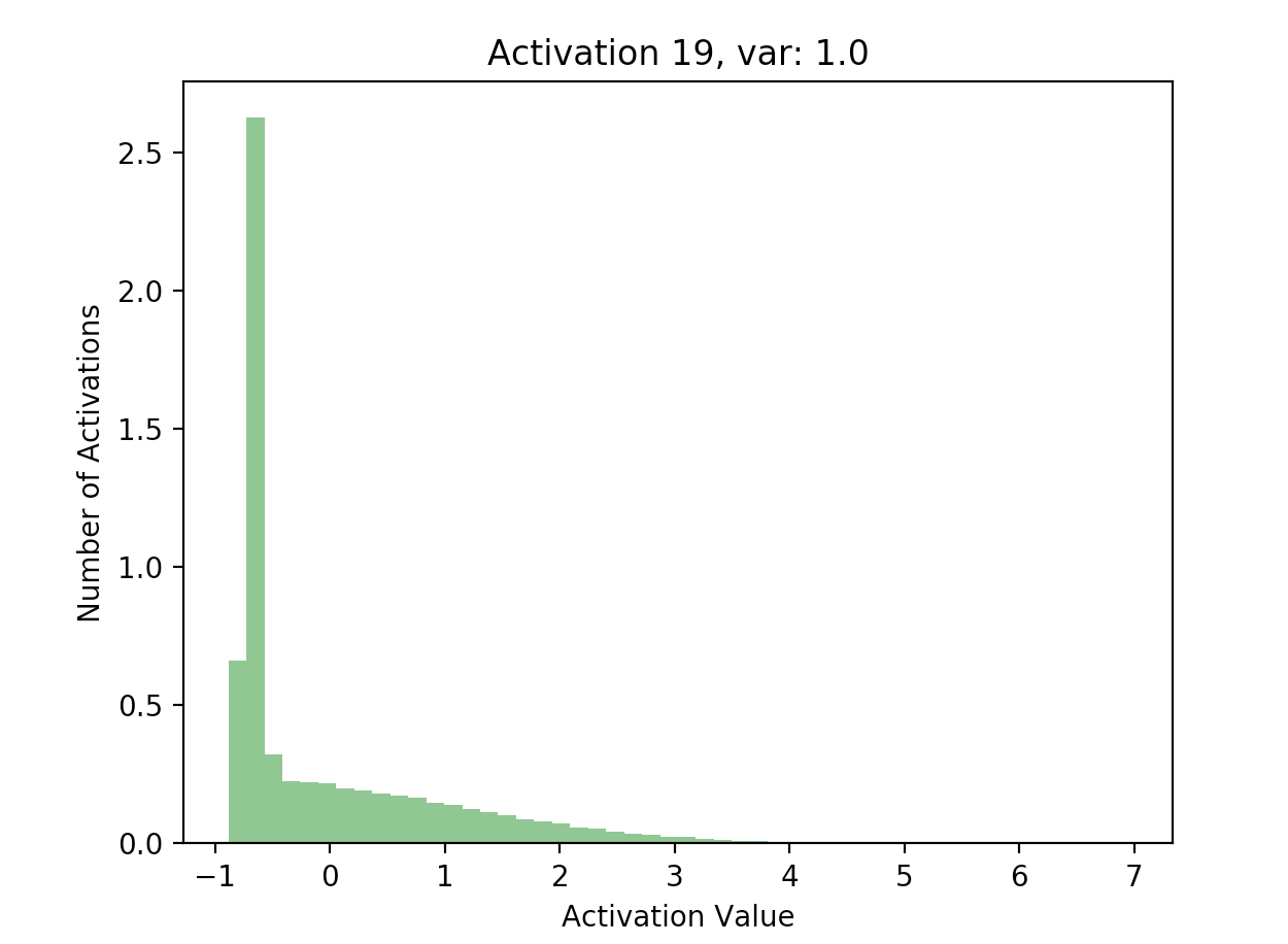
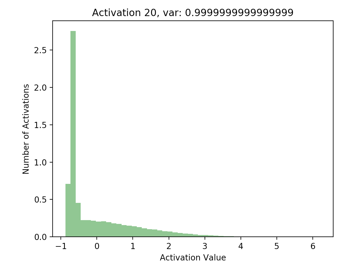
Now that we have a list of each layer’s hidden activations stored in hs, we can go ahead and plot the activations to see what their distribution looks like. Here, I’ve included plots of the activations at the first and final hidden layers in our 20 layer network:

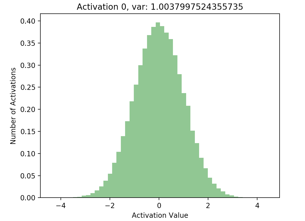
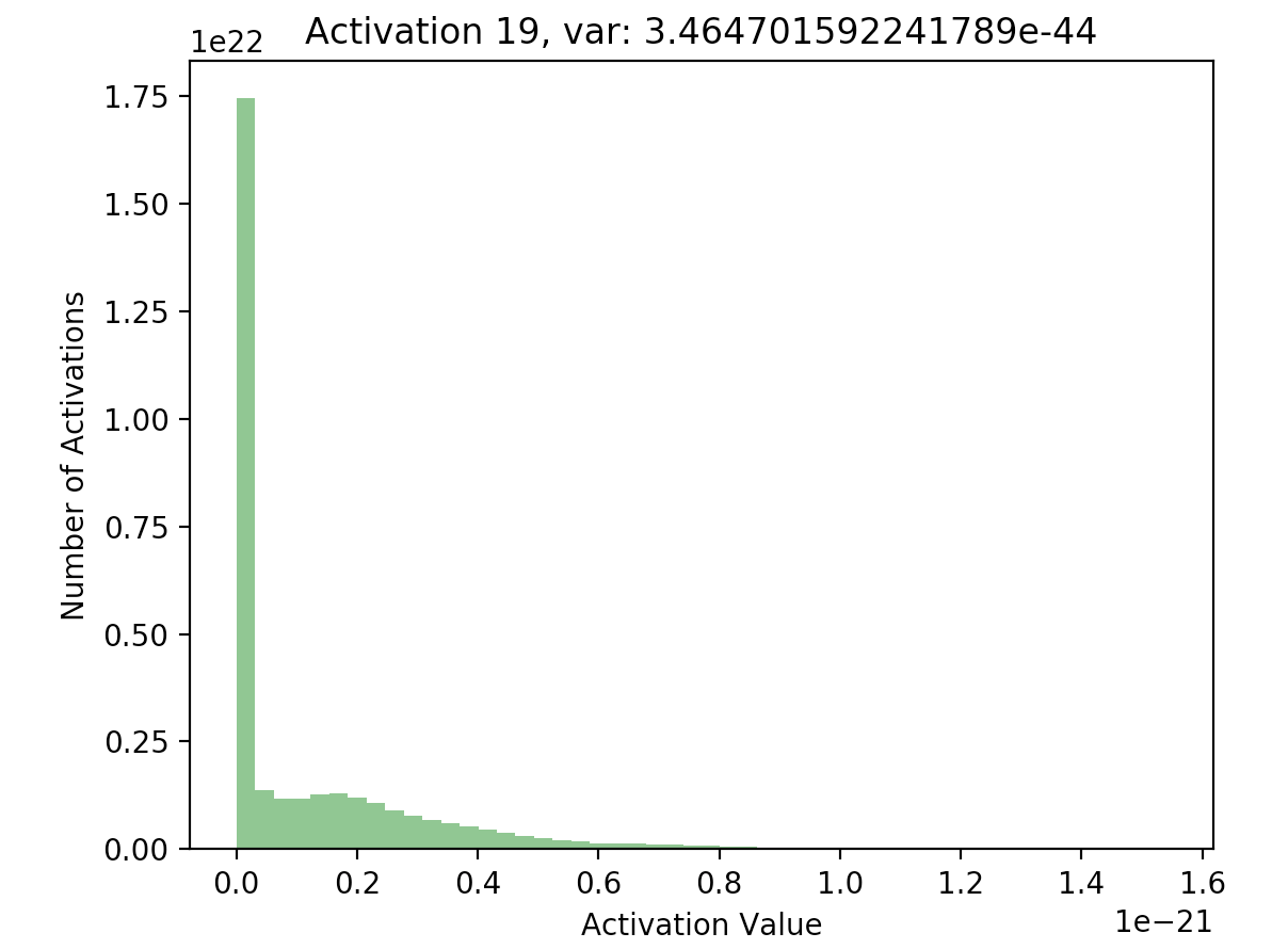
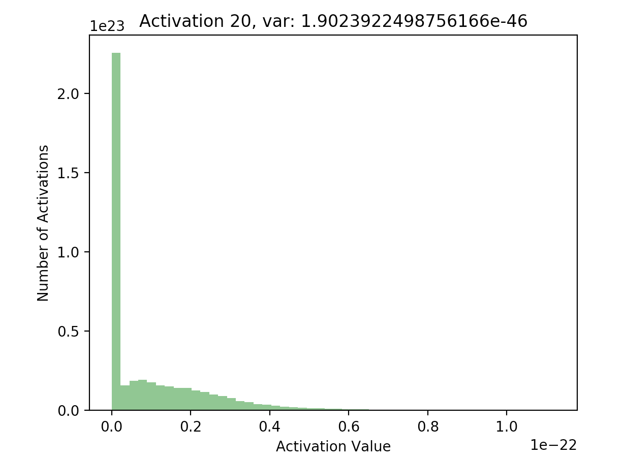
What’s important to notice is that in later layers, nearly all of the activations are zero (just look at the scale of the axes). If we look at the distributions of these activations, it’s clear that they differ significantly with respect to each other - the first activation takes on a clear Gaussian shape around 0, while successive hidden layers have most of their activations at 0, with rapidly decreasing variance. This is what the batch normalization paper refers to as internal covariate shift - it basically means that the distributions of activations differ with respect to each other.

Why does this matter, and why is this bad?

This is bad mostly due to the small, and decreasing variance in the distributions of our activations across layers. Having zero activations is fine, unless nearly all your activations are zero. To understand why this is bad, we need to look at the backwards pass of our network, which is responsible for computing each gradient \(\frac{dL}{dW_i}\) across each hidden layer in our network. Given the following formulation of an arbitrary layer in our network: \(h_i=relu(W_ih_{i−1}+b_i)\) where \(h_i\) denotes the activations of the ith layer in our network, we can construct the local gradient \(\frac{dL}{dW_i}\). Given an upstream gradient into this layer \(\frac{dL}{dh_i}\), we can compute the local gradient with the chain rule:

Applying the derivatives, we obtain:

Concretely, we can take our loss function for a single point to be given by the squared error, i.e. \(L_i = \frac{1}{2}(y-t)^2\), and if we were at the last layer of our network (i.e. \(h_i = y\)), our upstream gradient would be \(\frac{dL}{dh_i} = h_i - t\). This would give us a gradient of

in the final layer of our network.

What does this tell us about our gradients for our weights?

The expression for the gradient of our weights is intuitive: for every element in the incoming gradient matrix, pass the gradient through if this layer’s linear transformation would activate the relu neuron at that element, and scale the gradient by our input into this layer. Otherwise, zero out the gradient.

This means that if the incoming gradient at a certain element wasn’t already zero, it will be scaled by the input into this layer. The input in this layer is just the activations from the previous layer in our network. And as we discussed above, nearly all of those activations were zero.

Therefore, nearly all of the gradients backpropagated through our network will be zero, and few weight updates, if any, will occur. In the final few layers of our network, this isn’t as much of a problem. We have a strong gradient signal (i.e. \(h_i - t\) in the example above) coming from the gradient of our loss function with respect to the outputs of our network (since it is early in learning, and our predictions are inaccurate). However, after we backpropagate this signal even a few layers, chances that the gradient is zeroed out become extremely high.

In order to see if this is actually true, we can write out the backwards pass of our 20 layer network, and plot the gradients as we did with our activations. The following code computes the gradients using the expression given above, for all layers in our network:

dLdh = 100 * np.random.randn(hidden_layer_dim, input_dim) # random incoming grad into our last layer
h_grads = [dLdh] # store the incoming grads into each layer
w_grads = [] # store dL/dw for each layer

for i in np.flip(np.arange(1, n_layers), axis = 0):
	# get the incoming gradient
	incoming_loss_grad = h_grads[-1]
	# backprop through the relu
	dLdz = incoming_loss_grad * (zs[i] > 0) # zs was the result of Wx + b
	# get the gradient dL/dh_{i-1}, this will be the incoming grad into the next layer
	h_grad = ws[i-1].T.dot(dLdz) # ws[i-1] are our weights at this layer
	# get the gradient of the weights of this layer (dL/dw)
	weight_grad = dLdz.dot(hs[i-1].T) # hs[i-1] was our input into this layer
	h_grads.append(h_grad)
	w_grads.append(weight_grad)

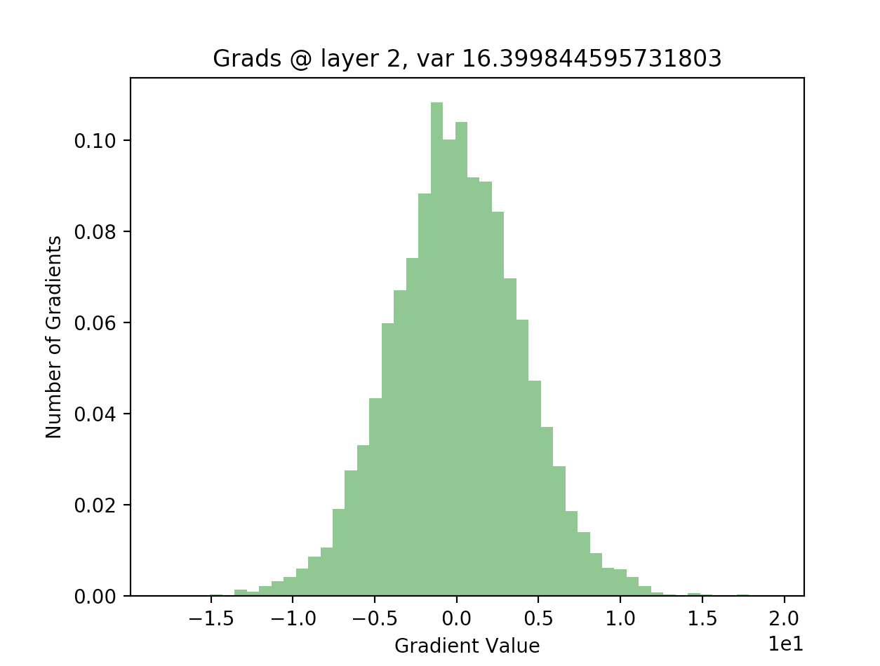
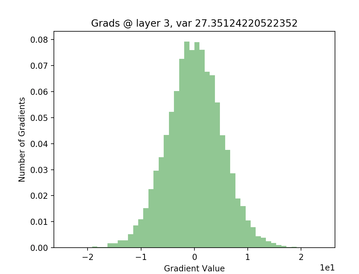
Now, we can plot our gradients for our earlier layers and see if our hypothesis was true:

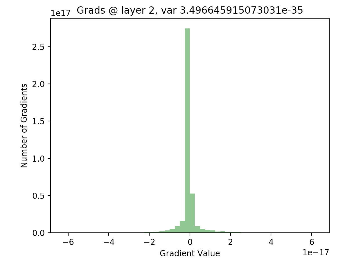
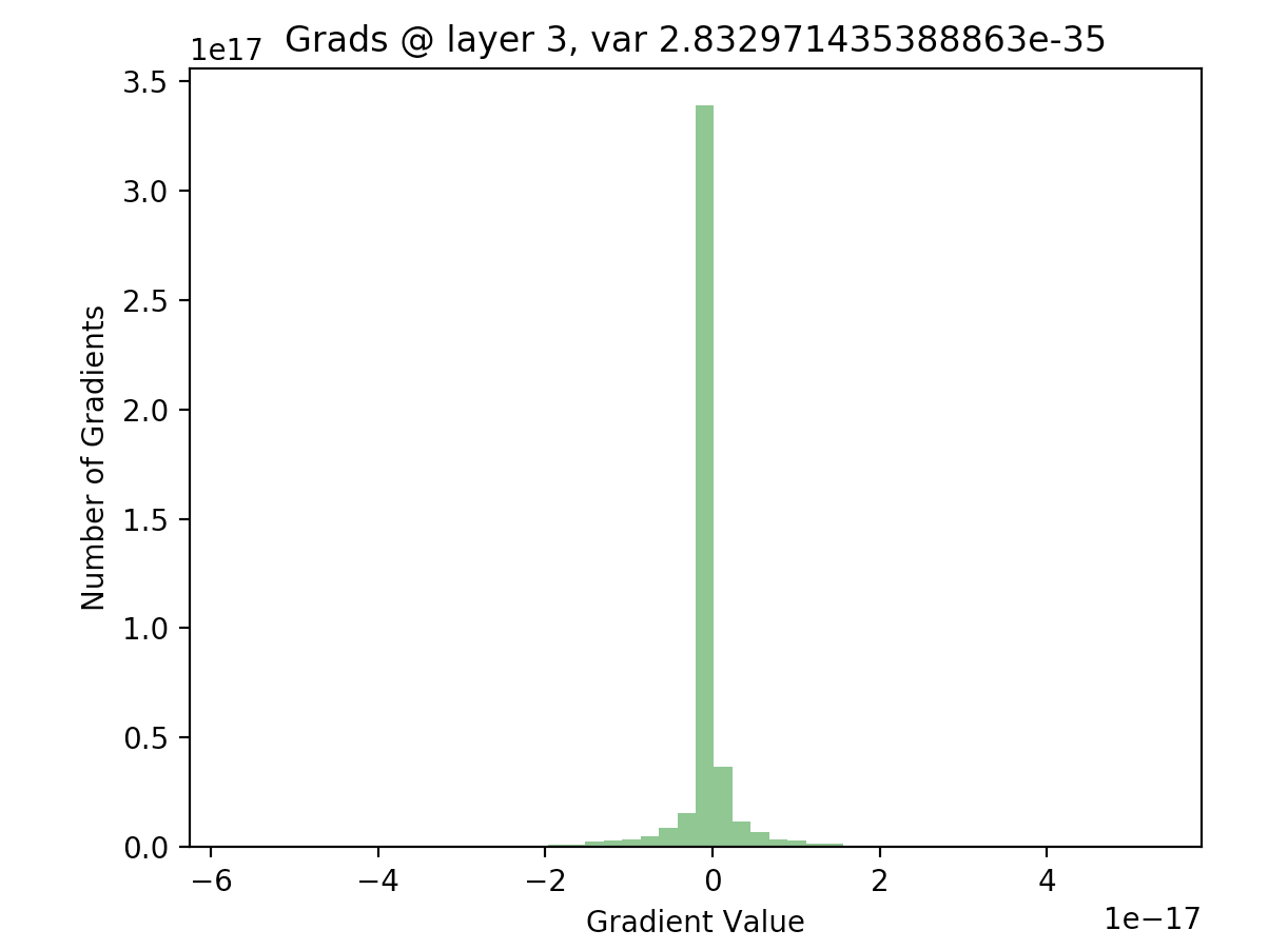
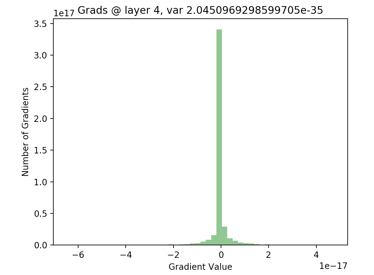
As we can see, for the final layer vanishing gradients aren’t an issue, but they are for earlier layers - in fact, after a few layers nearly all of the gradients are zero). This will result in extremely slow learning (if at all).

Ok, but what does batch normalization have to do any of this?

Batch normalization is a way to fix the root cause of our issue of zero activations and vanishing gradients: reducing internal covariate shift. We want to ensure that the variances of our activations do not differ too much from each other. Batch normalization does this by normalizing each activation in a batch:

Here, we denote\(x_k\) to be a certain activation, and \(\mu_B\), \(\sigma^2_B\) to be the mean and variance across the minibatch for that activation. A small constant \(\epsilon\) is added to ensure that we don’t divide by zero.

This constrains all hidden layer activations to have zero mean and unit variance, so the variances in our hidden layer activations should not differ too much from each other, and therefore we shouldn’t have nearly all our activations be zero.

It’s important to note here that batch normalization doesn’t force the network activations to rigidly follow this distribution at all times, because the above result is scaled and shifted by some parameters before being passed as input into the next layer:

This allows the network to “undo” the previous normalization procedure if it wants to, such as if \(y_k\) was an input into a sigmoid neuron, we may not want to normalize at all, because doing so may constrain the expressivity of the sigmoid neuron.

Does normalizing our inputs into the next layer actually work?

With batch normalization, we can be confident that the distributions of our activations across hidden layers are reasonably similar. If this is true, then we know that the gradients should have a wider distribution, and not be nearly all zero, following the same scaling logic described above.

Let’s add batch normalization to our forward pass to see if the activations have reasonable variances. Our forward pass changes in only a few lines:

n_examples, hidden_layer_dim = 100, 100
input_dim = 1000
X = np.random.randn(n_examples, input_dim) # 100 examples of 1000 points
n_layers = 20
layer_dim = [hidden_layer_dim] * n_layers # each one has 100 neurons

hs = [X] # save hidden states
hs_not_batchnormed = [X] # saves the results before we do batchnorm, because we need this in the backward pass.
zs = [X] # save affine transforms for backprop
ws = [] # save the weights
gamma, beta = 1, 0
# the forward pass
for i in np.arange(n_layers):
	h = hs[-1] # get the input into this hidden layer
	W = np.random.normal(size = (layer_dim[i], h.shape[0])) * 0.01 # weight init: gaussian around 0
	z = np.dot(W, h)
	h_out = z * (z > 0)
	# save the not batchnormmed part for backprop
	hs_not_batchnormed.append(h_out)
	# apply batch normalization
	h_out = (h_out - np.mean(h_out, axis = 0)) / np.std(h_out, axis = 0)
	# scale and shift
	h_out = gamma * h_out + beta
	ws.append(W)
	zs.append(z)
	hs.append(h_out)

Using the results of this forward pass (again stored in hs), we can plot a few of the activations:

This is great! Our later activations now have a much more reasonable distribution compared to previously, where they were all almost zero - just compare the scales of the axes on the batchnorm graphs against the non-original graphs.

Let’s see if this makes any difference in our gradients. First, we have to rewrite our original backwards pass to accommodate the gradients for the batchnorm operation. The gradients I used in the batchnorm layer are the ones given by the original paper. Our backwards pass now becomes:

dLdh = 0.01 * np.random.randn(hidden_layer_dim, input_dim) # random incoming grad into our last layer
h_grads = [dLdh] # incoming grads into each layer
w_grads = [] # will hold dL/dw_i for each layer

# the backwards pass
for i in np.flip(np.arange(1, n_layers), axis = 0):
	# get the incoming gradient
	incoming_loss_grad = h_grads[-1]
	# backprop through the batchnorm layer
	#the y_i is the restult of batch norm, so h_out or hs[i]
	dldx_hat = incoming_loss_grad * gamma
	dldvar = np.sum(dldx_hat * (hs_not_batchnormed[i] - np.mean(hs_not_batchnormed[i], axis = 0)) * -.5 * np.power(np.var(hs_not_batchnormed[i], axis = 0), -1.5), axis = 0)
	dldmean = np.sum(dldx_hat * -1/np.std(hs_not_batchnormed[i], axis = 0), axis = 0) + dldvar * -2 * (hs_not_batchnormed[i] - np.mean(hs_not_batchnormed[i], axis = 0))/hs_not_batchnormed[i].shape[0]
	# the following is dL/hs_not_batchnormmed[i] (aka dL/dx_i) in the paper!
	dldx = dldx_hat * 1/np.std(hs_not_batchnormed[i], axis = 0) + dldvar * -2 * (hs_not_batchnormed[i] - np.mean(hs_not_batchnormed[i], axis = 0))/hs_not_batchnormed[i].shape[0] + dldmean/hs_not_batchnormed[i].shape[0]
	# although we don't need it for this demo, for completeness we also compute the derivatives with respect to gamma and beta. 
	dldgamma = incoming_loss_grad * hs[i]
	dldbeta = np.sum(incoming_loss_grad)
	# now incoming_loss_grad should be replaced by that backpropped result
	incoming_loss_grad = dldx
	# backprop through the relu
	print(incoming_loss_grad.shape)
	dLdz = incoming_loss_grad * (zs[i] > 0)
	# get the gradient dL/dh_{i-1}, this will be the incoming grad into the next layer
	h_grad = ws[i-1].T.dot(dLdz)
	# get the gradient of the weights of this layer (dL/dw)
	weight_grad = dLdz.dot(hs[i-1].T)
	h_grads.append(h_grad)
	w_grads.append(weight_grad)

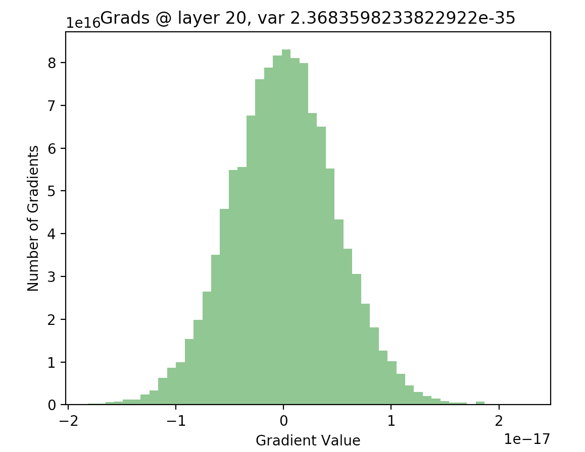
Using this backwards pass, we can now plot our gradients. We expect them to no longer be nearly all zero, which will mean that avoiding internal covariate shift fixed our vanishing gradients problem:

Awesome! Looking at our gradients early in the network, we can see that they follow a roughly normal distribution with plenty of non-zero, large-magnitude values. Since our gradients are much more reasonable than previously, where they were nearly all zero, we are more confident that learning will occur at a reasonable rate, even for a large deep neural network (20 layers). We’ve successfully used batch normalization to fix one of the most common issues in training deep neural networks!

Intuition for why Batch Normalization helps with better gradient signals

When gradient descent updates a certain layer in our network with the gradient \(\frac{dL}{dW_i}\), it is ignorant of the changes in statistics in other layers - for example, it implicitly assumes that the distribution of the activations of the previous layer (and hence the input into this layer) stay the same as it updates the current layer it is on. Without batch normalization, this assumption isn’t true: gradient descent also eventually updates the weights in the previous layer, therefore changing the statistics of the output activations for that layer. Therefore, there could be a case where we update layer \(i\) , but the distribution of the inputs into that layer change such that the update actually does worse on these new inputs. Batch normalization fixes this, by guaranteeing that the statistics of the input into each layer stay the same throughout the learning process. See this explanation by Goodfellow for more on this.

P.S. - all the code used to generate the plots used in this answer are available here.

References

1. Batch Normalization Paper
2. CS 231n Lecture on Batch Normlization

Notes

[2/19/18] - I originally wrote this as an answer on Quora

[2/21/18] - The code used in the forward and backward pass isn’t completely accurate with respect to scaling the outputs by parameters \(\gamma\) and \(\beta\). In actuality, there is supposed to be a \(\gamma_i\) and a \(\beta_i\) for each activation in each hidden layer - for example, if we have a batch of \(n\) activations and each activation has shape \(1000\), there should be \(1000\) \(\gamma_i\)s and \(1000\) \(\beta_i\)s in each layer. I didn’t bother to actually implement it this way as it doesn’t affect the normalization process for the one step I illustrated.

[2/22/18] - I applied batch normalization after the ReLU nonlinearity, whereas the original paper states that it is applied after the affine layer and before the nonlinearity. Apparently, their actual code applies it after the ReLU as well, and it was mis-stated in their paper. See this Reddit thread for more discussion.