
ResNet Paper Notes
ResNet paper notes
These are some notes that I took while reading the paper Deep Residual Learning for Image Recognition, the paper that introduced modern ResNets.
1. Introduction
-
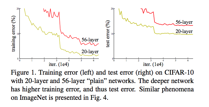
Main motivation: very deep neural networks are harder to fit
-
Have higher training error on CIFAR 10 - so learning is not as simple as stacking more layers as it was once thought
-
Degredation problem is because it is difficult to fit very deep networks (despite batch normalization and He/Xavier initialization methods), they don’t just overfit, they actually have worse training error
-
-
Intuitively, deep networks should’t be “harder” to fit. If there is a certain number of layers \(N\) that achieve optimal accuracy on a dataset, then the layers after N could just learn the identity mapping (i.e. each layer computes their mapping as \(H(x) = x\) where \(H(x)\) is the mapping of the layer to be learned), and then the network will effectively have their final output at layer \(N\)
-
However, it is not “easy”for weights to be pushed in such ways that they exactly produce the identity mapping
-
Authors introduce the idea of residual learning - instead of directly approximating the underlying mapping we want, \(H(x)\), we instead learn a residual function \(H(x) - x\). This is done by making the output of a stack of layers be \(y = F(x) + x\), where \(F(x)\) is the output of the layers (before the ReLU of the last layer) and then the original input \(x\) is element-wise added:
-
Therefore, if our underlying mapping is still \(y = H(x)\) that we want to learn, then \(F(x) = H(x) - x\) so that \(y = F(x) + x = H(x) - x + x = H(x)\) .
- The idea of learning identity mappings is now easier, since we just need to set all weights to \(0\), so that \(H(x) = 0\) and \(F(x) = -x\), so \(y = x\) is learned
-
Ensemble of ResNets attained 3.57% top-5 error rate on ImageNet dataset
- Six total ResNets of different dimension, 2 152-layer ResNets are used
2. Related Work
- Auxiliary classifiers inserted at early layers of a deep network to send back stronger gradient signals to deal w/vanishing gradient problems are similar
- Inception network which uses concatenations of different operations includes a shortcut connection
3. Deep Residual Learning
-
Say we want to learn \(y = H(x)\). We can either cdirectly learn this or try to learn \(F(x)\) where \(F(x)= H(x)-x\) and formulate our output as \(y = F(x) + x\). So by addign the identity in a so-called “residual block” we force the nework to learn a residual mapping \(F(x) = H(x) -x\).
-
A building block in ResNet is defined as \(y = F(x_i, {W_i}) + x\) where \(F\) can be multiple layers. For example, the above figure has \(F = W_2(\sigma (W_1 x))\)
- The \(+\) operation is performed by a shortcut operation and element-wise addition
-
Described like this, the shortcut connection introduces no new parameters in a network, so training the network in this way doesn’t introduce an increase in training time due to the numbers of parameters that must be trained. But this isn’t possible when dimensionalities are different - for example, the 2 layers of conv/relu above may result in the output before the addition having different dimension than that of \(x\).
-
To handle this, we can use a projection matrix \(W_s\) that projects \(x\) to the same space as \(F(x)\). We have \(y = F(x, {W_i}) + W_sx\), but this introduces more parameters into the network.
-
These functions are just as applicable to convlutional layers as they are to FC layers. For examples, \(F\) can represent multiple conv layers, and the element-wise addition is performed on the two feature maps, going channel by channel (so the dims must be the same)
-
Residual Network details
-
Based off a plain 34-layer network that has a \(7 * 7\) conv, then a series of \(3*3\) convs gradually increasing the channel size, followed by a global average pooling layer, followed by a \(1000\) way FC layer + softmax at the end that represents \(p(y \vert{} x)\)
-
The residual network is similar , but shortcut connectins are added every 2 layers, and the network looks as follows:
-
Two options when dimensions don’t map:
- Projection matrix (as mentioned above), or just padding extra zeros to increase dimension (doesn’t increase number of parameters) are both tried out
-
Downsampling is directly performed with the stride size, which is \(2\) in all of the conv layers.
-
Design rules: If the output of a conv layer has the same feature map size, the layers have the same number of filters, but if the size of the feature map is halved, then the number of filters is doubled, so as to preserve the time complexity per layer.
-
Implementation details:
- 224 x 224 crops sampled from ImageNet dataset, with per-pixel mean subtracted
- Data augmentation: images are flipped to increase dataset size
- Batch norm is used, the pattern is conv-bn-relu, so before the activation
- He initialization of weights is used, namely weights are initialized from sampling from a Gaussian with mean \(0\) and standard deviation \(\sqrt{\frac{2}{n_l}}\). Biases are initialized to be \(0\).
- SGD with minibatch size 256 is used
- Learning rate starts off as \(0.1\) and is then decreased by dividing by \(10\) when the error plateus.
- \(60 * 10^4\) total iterations
- Weight decay of \(0.0001\) and momentum of \(0.9\) is used
- Dropout is not used, in favor of only batchnorm.
-
4. Training and Approach
-
Trained 18 and 34 layer plain networks, along with 18 and 34 layer ResNets
- It was shown that 34 layer plain nets have higher training error than 18 layer nets, and it was argued that this was not due to vanishing gradients, because: 1) proper initialization was used, 2) BN was used, 3) it was ensured that gradients have healthy norms throughout training
- Speculated that deep networks have exponentially lowe convergence rates (i.e. need to be trained for much longer to achieve same results compared to shallower networks)
-
For 18 and 24 layer ResNets, simple element-wise addition shortcut additions were used, so there were no new parameters in the network
- 34 layer ResNet did better compared to 18 layer, indicating that the degredation problem observed in shallow nets was not evident here
-
Identity vs projection shortcuts
- 3 types:
- A: zero-padding shortcuts used when dimensions do not match, all shortcuts are parameter free
- B: Projection shortcuts used when dimensions do not match, and other shortcuts are regular element-wise addition
- C: All shorcuts are projections (meaning that a square matrix is used even when the dimensions match)
- It was shown that B is slightly better than A and C was slightly better than B, but C introduces more parameters and increases the time/memory complexity of the network, so B was used overall (projections when dimensions do not match, otherwise regular identity and element-wise addition)
- 3 types:
-
Bottleneck architecture
-
For every residual function \(F\), 3 layers instead of 2 are used: first layer is a 1x1 conv, then a 3x3 conv, then a 1x1 conv
- The 1x1 layers reduce and increase dimensionality, and the 3x3 conv operates on a smaller dimensional space
-
Exampe: in the following figure, a \(256\) dimensional (256 channels) input is fed into a 1x1 which maps it to 64 channels, then a 3x3 which maps it to 64 channels, and then 1 x 1 that maps it back to the original dimensionality of 256 channels.
-
Parameter-free shortcuts here are particularly important, the time complexity and model size are doubled if identity shortcuts are replaced with projection
-
This architecture is used to create 50/101/152 layer ResNets, which all had improved accuracy compared to the 34 layer ResNets, and the degredation problem is not observed
- 152-layer ResNet performed the best
-
ResNets on CIFAR-10
- Network inputs are 32 * 32 with per-pixel mean subtracted
- First layer: 3 x 3 conv, then stack of \(6n\) layers with \(3*3\) convolutions with feature map sizes of 32, 16, and 8. Each feature map size has \(2n\) layers for \(6n\) total layers.
- This means that the output feature map size is 32 twice, then 16 twice, etc
- Number of filters are 16, 32, 64, respectively. Subsampling is done with conv layers of stride 2 instead of max/average pooling throughout the network (which is the traditional way of downsampling)
- Global average pooling after all the conv layers, and then a 10-way fully connected layer + softmax at the end
- Identity shortcuts used in all cases
- Weight decay: \(0.0001\), momentum of \(0.9\), with He init, BN, and no dropout, with a batch size of \(128\).
- Learning rate of \(0.1\) which is divided by \(10\) at 32k and 48k iterations, and training is terminated at 64k iterations
- 110 layer network achieved \(6.43\)% error, which is state of the art
- Noticed that deeper ResNets have a smaller magnitute of responses, where a response is the standard deviation of layer responses for each layer (i.e. the responses in layers of the ResNets generally have lower standard deviations compared to plain networks)
- 1202 layer network did not work well (had similar training error, but higher testing error, indicatign overfitting)
- Not much regularization was used in these ResNets (i.e. no maxout or dropout), regularization is just imposed by the architecture of the design